Google Sheets scripting
Created: 2019-08-11 20:22:27 -0700 Modified: 2019-08-18 17:24:56 -0700
Basic scripting
Section titled “Basic scripting”- Google Apps Script is just JavaScript (reference).
- At the time of writing (8/11/2019), “let” and string interpolation don’t work. const does not work how you expect from ES6 (it doesn’t seem to be block-scoped, so don’t use it within loops).
- When you share a sheet with “Edit” permissions, they get edit access to any scripts you may have written. They also need to accept permissions in the Sheet for the script. You’ll both be modifying the same script, but you don’t see changes in realtime, so IMO, it’s a bad idea to try to edit scripts concurrently.
- API documentation for Sheets is here.
- Handy pages
- Sheet
- Cells (AKA ranges, since a single cell is just a small Range)
- Utilities.formatDate
- Handy pages
- You can develop locally using clasp (takes roughly 2 minutes to set up):
- Allow Google Apps Script API here: https://script.google.com/home/usersettings (or else “clasp push” will give a 403)
npm install @google/clasp -gclasp login- This pops up an OAuth webpage
- clasp clone <script ID found from File → Project properties → Info → Script ID>
- Modify files locally
clasp push
- In general, let the sheet do the heavy lifting via formulas rather than scripting everything. For example, if you need to sum a bunch of rows that aren’t moving anywhere, then just do something like =SUM(C2:C5). By doing things this way, they’ll always be up-to-date despite changes to the referenced cells.
- Triggers are in found in the script’s Edit → Current project’s triggers → Add trigger (reference). They can run a function on a certain event, e.g. opening a document or editing a cell’s value.
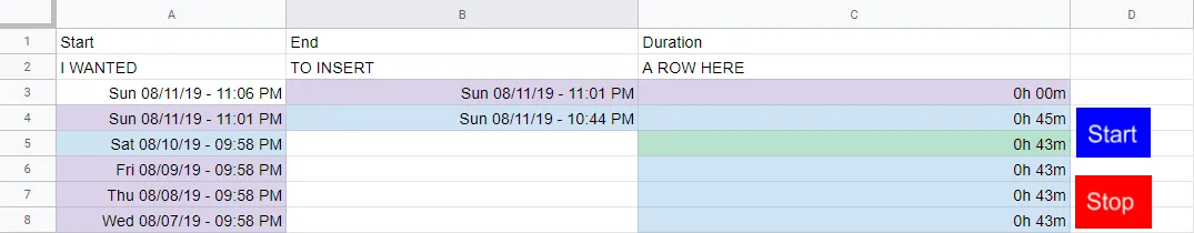
- I originally wanted to show an up-to-date time like a stopwatch, but rather than doing that through a script, I decided to try it through the built-in formulas. File → Project settings → Calculation → Recalculation → On change and every minute. Then, I made a formula like =(NOW() - A2)
- If you have a Date in a cell and you want to format it with the total number of hours, it’s represented via
[h]. “h” without square brackets cannot exceed 23 (reference). As far as I can tell, you cannot do this with elapsed days. - Sheets treats Dates in units of days. This means that “1” represents 24 hours, “0.25” is 6 hours, etc.:
- Whenever you subtract two Date objects, you get another Date object that looks like it’s in 1970 just because it represents the number of milliseconds that have elapsed. In the debugger, it’ll look like this:
- If you ever need to compare that time via a Google Apps Script, use date.getTime().
- Whenever you subtract two Date objects, you get another Date object that looks like it’s in 1970 just because it represents the number of milliseconds that have elapsed. In the debugger, it’ll look like this:
Basic examples
Section titled “Basic examples”- Get the active sheet:
const sheet = SpreadsheetApp.getActiveSheet(); - Set a single cell’s contents
sheet.getRange('A2').setValue('Foo')sheet.getRange('A2').setFormula('=NOW()')
- Pop up a message box:
Browser.msgBox("testeroni"); - Convert from a formula to a value:
sheet.getRange('A2').setValue(sheet.getRange('A2').getValue());- You can use this immediately after calling setFormula, e.g.
var a = activeSheet.getRange('F4').setFormula('=SUM(F2:F3)').getValue()
- You can use this immediately after calling setFormula, e.g.
- Inserting a single cell: this isn’t possible (reference)
-
When I wanted to add a row that just spanned three columns, I did this:
activeSheet.getRange("A2:A").moveTo(activeSheet.getRange("A3"));activeSheet.getRange("B2:B").moveTo(activeSheet.getRange("B3"));activeSheet.getRange("C2:C").moveTo(activeSheet.getRange("C3"));- Note: if I’d been okay inserting a whole row, I could have done this
-
Converting from a number to a letter (e.g. 1 → A, 52 → AZ) (reference)
Section titled “Converting from a number to a letter (e.g. 1 → A, 52 → AZ) (reference)”Use these functions from the reference link:
function columnToLetter(column){  var temp, letter = '';  while (column > 0)  {    temp = (column - 1) % 26;    letter = String.fromCharCode(temp + 65) + letter;    column = (column - temp - 1) / 26;  }  return letter;}
function letterToColumn(letter){  var column = 0, length = letter.length;  for (var i = 0; i < length; i++)  {    column += (letter.charCodeAt(i) - 64) * Math.pow(26, length - i - 1);  }  return column;}
Adding a button (reference)
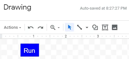
Section titled “Adding a button (reference)”- Insert → Drawing. Note: it doesn’t matter which cells/rows you have selected since the drawing gets added sort of on top of everything.
- Make a button. I just made a textbox, changed the colors, and wrote “Run”
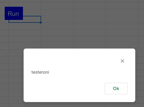
- Tools → Script editor
- In “myFunction”, add Browser.msgBox(“testeroni”);
- Test this via Run → Run function → myFunction
- You may have to save the script and grant permissions
- The message box shows back in the Sheets tab of your browser, not the scripts tab
- Back in the sheet, right-click your button, click the three dots, and choose Assign script → myFunction (you have to type it in).
- Click your button to test it:
- After clicking a button, even something like
sheet.getRange("B2").activate()will have the focus on the button. There is no programmatic way around this; you need to press escape on the keyboard to get the focus off of the button (reference).
Troubleshooting
Section titled “Troubleshooting”Service error: Spreadsheets
Section titled “Service error: Spreadsheets”
Apparently this is the “oh no, you figure it out” error. In my particular case, I had this code:
activeSheet.getRange("C2:C").moveTo(activeSheet.getRange("C3"));I think the problem was that I had another cell (in the middle of nowhere) with the formula “=SUM(C2:C)”, so attempting to move C2:C caused a problem for some reason. Potential workarounds:
- Moving C3:C instead of C2:C
- Disabling the formula in the random cell
- Calling insertRowAfter instead of moveTo (although this has different semantics since it makes a new row in EVERY column, not just in C)