Dynamic programming

Created: 2020-07-18 14:24:44 -0700 Modified: 2020-08-01 21:26:35 -0700

Dynamic programming

I’m taking these notes based on this MIT video series:

All videos are part of the Introduction to Algorithms course unit 7 (the “unit 7” shows on the Lecture Notes page).

Terminology:

DP: dynamic programming
DAG: directed acyclic graph
Indegree (reference): the number of head ends (i.e. the number of incoming edges) adjacent to a vertex is the indegree of the vertex
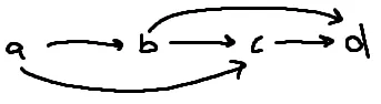
Topological sort (reference): for a DAG, this is an order that guarantees that for every edge from X to Y in the graph, X will always show up before Y. For example, this graph’s topological sort can only be [A,B,C,D]:

My summary of everything after having watched all four videos

(note: there will be overlap here with the individual videos’ notes)

Five steps to DP:

Define subproblems
1. This typically involves either:
  1. Prefix (or suffix): O(N) time
  2. Substring: O(N²) time
Guess some part of the solution
1. Do we take this index? If so, does it increase our cost by some number?
2. Is this a base case (in which case maybe we know the output for that base case)?
Relate subproblem solutions to each other (it’s typically a minimum or maximum of the subproblems)
Build the algorithm (top-down: recurse + memoize, bottom-up: build a DP table)
Make sure you’ve solved the original problem

Time complexity: #subproblems * time per subproblem (usually polynomial).

My realizations after testing all of this

If the way you defined your recurrence doesn’t end up using a subproblem to solve another problem, then you just have a recurrence, not a relation. This means that you can use recursion but probably not DP unless you change your subproblems.
- For example, if you just want to find all nodes in a graph, you’d use DFS or BFS. Neither is really DP.
- As another example, consider the maximum-subarray problem, something typically solved by Kadane’s Algorithm in O(N) time. The DP way of solving this doesn’t actually use subproblems in the conventional sense; you would have something like this:

(l = left, r = right)
  dp[l, r] = max(
    getSum(l, r),
    dp[l+1, r],
    dp[l, r-1]
  )

As you can see, we’re just taking the maximum possible sum of every single subarray without reusing anything, so we’ll do this in O(N²) since the number of subproblems is N, and getSum operates in O(N) time (N * N = N²).

What we could reuse for a slice of N elements is N-1 elements on the left or right if that sum>0, otherwise it won’t contribute to the largest sum.

Video 19 - Fibonacci, shortest paths (reference)

Basics

Overview
- DP is good for minimizing, maximizing, shortest paths, etc.
- It’s splitting problems into subproblems and reusing their solutions
  - Thus, he says that dynamic programming is roughly recursion + memoization
- He generalizes this in video 2 to say that DP problems can almost always be simplified down to shortest paths in some DAG. Later, in video 3, he says that it’s not always the case.
Time complexity
- You typically get polynomial time even when doing an exhaustive search thanks to memoization
  - The time complexity is: #subproblems * time/subproblem

Fibonacci examples

Recursive algorithm without DP

To compute the nth Fibonacci number:

fib(n):
  if n ≤ 2: return 1
  else: return fib(n-1) + fib(n-2)

Time complexity: exponential. He drew out a tree showing this:

To compute f(n), you need to compute f(n-1) and f(n-2)
- To compute f(n-1), you need f(n-2) and f(n-3)
  - …so on
- To compute f(n-2), you need f(n-3) and f(n-4)
  - …so on

Memoized DP algorithm (top-down approach)

This is top-down because we’re starting at N and working our way down toward the base cases:

memo = {}
fib(n):
  if n in memo: return memo[n]
  f = 1
  if n > 2: f = fib(n-1) + fib(n-2)
  memo[n] = f
  return f

It’s pretty much the same as the recursive algorithm but with memoization. The memoized calls are done in constant time of course. The time complexity is linear.

Note: you can actually generate Fibonacci numbers in log(n) time by using 2D matrices, since f(n) = the matrix [[1,1][1,0]] ^ (n-1). He doesn’t discuss this in the video other than to point out that it’s possible.

The time complexity is: #subproblems * time/subproblem (ignore recursive calls in the time since you're memoizing their results).

Bottom-up DP algorithm

This is bottom-up because we’re starting at our base cases and working up toward N:

get_num(n):
  fib = {}
  for k in range(1, n+1):
    if k ≤ 2: f = 1
    else: f = fib[k-1] + fib[k-2]

    fib[k] = f

  return fib[n]

This is still solving all subproblems from 1 to n and then returning the answer to the nth problem.

This approach does a topological sort of the subproblem dependency DAG:

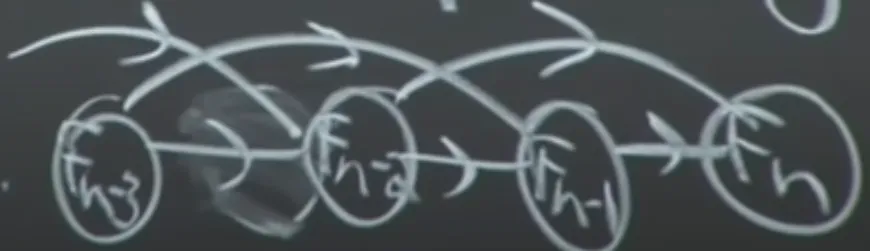
This shows us the order in which we’re supposed to solve the subproblems, which for Fibonacci is obvious since each one is based on the previous two.

Comparison between Fibonacci approaches

All three algorithms shown above use the same lines (well, not how I wrote them):

if k ≤ 2: f = 1
else: f = fib[k - 1] + fib[k - 2]

We can save space in the bottom-up approach since we only need to remember the last two values, not all of them starting at the base case. Thus, we only need constant space but still linear time.

Remember, with the top-down approach, it’s a little bit harder to see the time complexity, but it’s always #subproblems * time/subproblem.

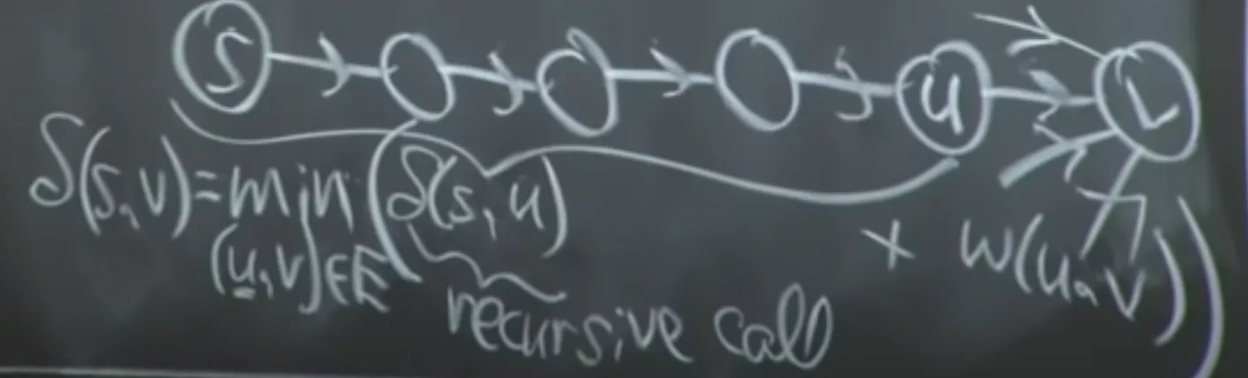
Shortest-path examples

We want to a shortest path from some node “s” to “v” for every “v” in the graph.

First, we consider the recursive solution. If we don’t know the solution, we can guess. More specifically, we can try all of the guesses (brute force) and then take the best one (and memoize it).

For shortest paths, we can start at the destination node and guess all of the possible incoming paths to “v”. We’ll find the best one, label it “u”, then find our shortest path from “s” to “u” (recursively).

If we didn’t get the right choice of u, then we have to guess again. We’re minimizing the choice of u.

This is exponential without memoization. We would memoize every path from S → X, where X is just some node (and since S doesn’t change, we just need to store the destinations in our memo table).

Even with memoization, this could be infinite if there are cycles:

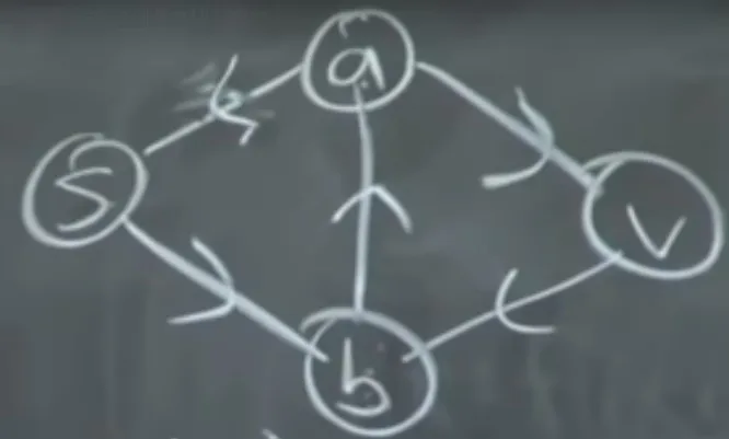
In this graph, there’s only one edge to V, which is A → V. There’s only one path to A, which is B → A. However, to get to B, we could have come from S or V. We would infinitely recurse if we came from V. So this technique only works for DAGs, in which case the time complexity is based on the number of vertices and number of edges.

This is where we go back to the topological sort of the sub-problem dependency DAG; we need some way to make a cyclic graph into an acyclic graph. He shows a technique for doing this, but he points out that it would change our time complexity since the number of subproblems is based on V², where V is the number of vertices in the graph.

This comes down to the Bellman-Ford algorithm, which I was unfamiliar with but shows up earlier in the course.

Video 20 - text justification, blackjack (reference)

Five steps to DP:

Define subproblems
Guess some part of the solution
Relate subproblem solutions to each other (it’s typically a minimum or maximum of the subproblems)
Build the algorithm (top-down: recurse + memoize, bottom-up: build a DP table)
Solve original problem

He says that the first two steps (figuring out the subproblems and figuring out what to guess) are the hard parts. After that, everything is essentially automatic.

In Fibonacci, there was nothing to guess since we only have two base cases, so we always start there. In the shortest-path problem, we had guessed one of the edges off of our target node, V.

Text justification

Split text into “good” lines such that you fit as many words as you can per line without leaving large spaces between words.

Input: list of words

There’s a “badness” function defined on a range [i..j] which indicates how bad it is to use words[i..j] as a line.

→ It returns infinity if the words don’t even fit

→ Otherwise, it returns (pageWidth - totalWidth)³. Cubing it makes it much worse to have large gaps.

To solve this, we have to find subproblems. It’s sometimes helpful to start by thinking of the brute-force strategy.

For every word, does it start a line or no? That’s our goal: to figure out where each line begins.

When we get which word starts each line, we can continue onward with the rest of the words (i.e. the suffix of the array). The subproblems here would be the suffixes, so we have n subproblems.

Blackjack

Assume you have perfect information, meaning you know the entire deck order.

No splitting, doubling, etc.

We have to figure out how many times we should hit.

Our guesses are going to try hitting 5 times, 1 time, etc.

The subproblems will be suffixes of the cards in the deck. We have perfect information, so we know the cards are c0, c1, …, cn-1. If we hit 0 times, then our suffix would be c[0..].

There are n subproblems.

The maximum number of hits is at most n - 4 since you deal 4 cards to begin with.

BJ(i) = max(outcome in {loss, tie, win}) + BJ(j) for number_of_hits in range (0, n) (if it’s a valid play; you can’t hit again if you’re above 21)

j = i + 4 + #hits + #dealer hits

The time complexity is cubic time (O(n³))

Video 21 - parenthesization, edit distance, knapsack (reference)

Note: for a string of length N, finding all possible substrings is O(N²) since you have to iterate over the string in two nested loops (e.g. ABC → A, B, C, AB, BC, ABC).

He says that considering prefixes (O(N)), suffixes (O(N)), and substrings (O(N²)) will get you through most DP problems. He also says that if you need both prefixes and suffixes, then you want substrings since they combine both.

Parenthesization

Optimal evaluation of associative expression, e.g. multiplying N matrices (matrix multiplication is not commutative).

A0 _ A1 _ … An-1

This can be changed into any combination of parentheses, e.g. ((A0A1)(A2*A3))

Some matrix multiplications are easier than others:

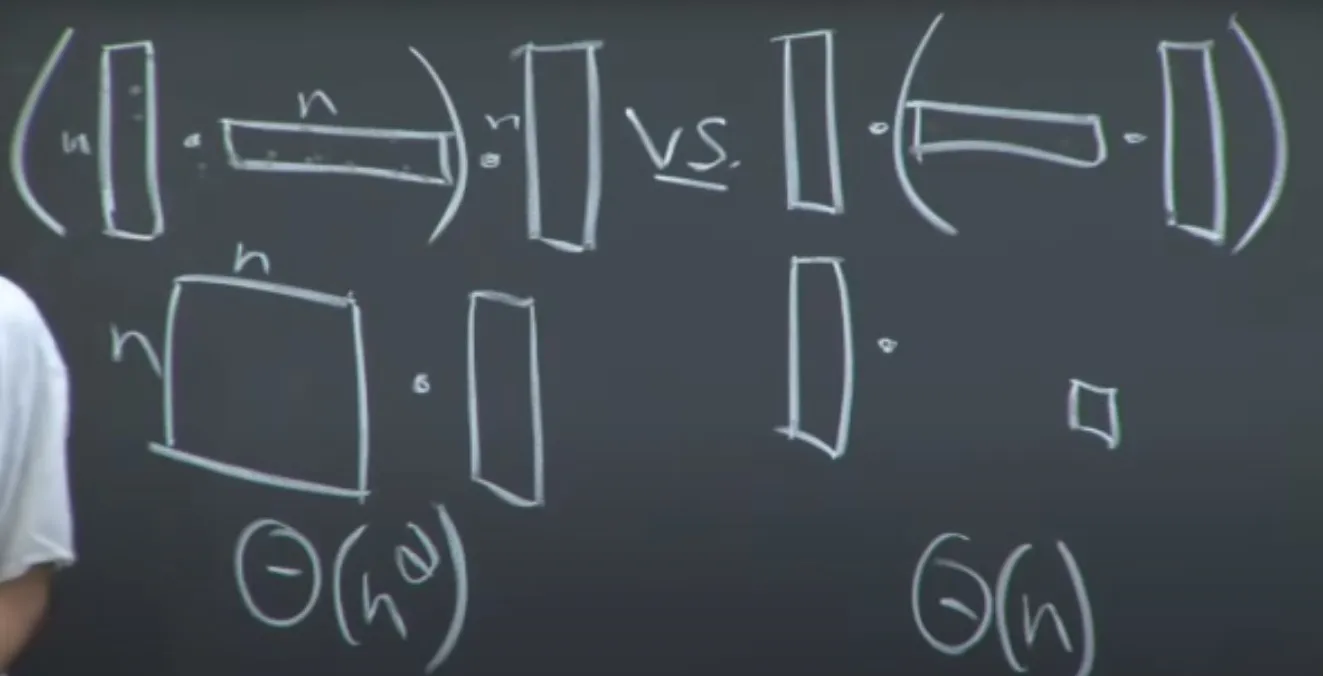
In the picture above, on the left, we multiply a column matrix by a row matrix and end up with a square matrix of NxN, which we then have to muliply by a column. However, if we had made the parentheses on the row and column first, then we end up with a single number.

To find the DP solution, we need to figure out what the subproblems are and what we should guess. We have to guess what the last operation we’re going to do, AKA the outermost multiplication.

Thus, our goal is to guess “k” where ((A0 to Ak-1) * (Ak to An-1)) is optimal. This now looks like a substring problem since we need to figure out the starting and ending values of k or k’.

Our subproblem is to find the optimal evaluation of some substring of the matrices Ai to Aj-1

DP(i,j) = min(

DP(i, k) + DP(k, j) + (cost of (Ai:k ) * (Ak:j ))

for k in range(i+1, j)

)

Time per subproblem: O(N)

#Subproblems: N² (because it’s a substring problem)

So total complexity: O(N³)

Note that there are about 4^N total parenthesizations, so DP is much better to use if you want to find the optimal way to multiply the matrices. Note that actually multiplying the matrices without assigning any parentheses may actually be more efficient, but that’s a trade-off where the cost of planning exceeds the cost of execution.

To do a topological sort for substrings, you can sort by string length, where the strings of length 0 are at the bottom of the DAG pointing up.

Edit distance

Given two strings X & Y, what’s the cheapest possible sequence of character edits to convert X → Y.

We can insert, delete, or replace a character.

Note that we may weight these based on likelihoods. For example, with regular typing, you may press “a” when you mean to press “s”, so the cost to replace an “a” with an “s” may be very low.

We’re trying to minimize the number of changes.

A similar problem is the longest common subsequence, e.g.

HIEROGLYPHOLOGY + MICHAELANGELO → HELLO or IEGLO

We can turn this into an edit-distance problem where we consider the cost to replace a character to be infinity (unless the characters are equal, in which case it’s 0).

Back to edit-distance problems: we can look at suffixes of both X and Y. Our subproblem will be to solve the edit distance on a suffix of X and Y: X[i:] and y[j:] for every i and j.

subproblems is n²

What are we guessing? Well, have three actions: insert, delete, and replace.

We could insert the right character (insert y[j] into X)

We could delete the wrong character (delete x[i])

We could replace it with the correct character (replace x[i] with y[j])

Our recurrence

DP(i, j) = min(

(cost of replace x[i] → y[j]) + DP(i+1, j+1),

(cost of insert y[j]) + DP(i, j+1),

(cost of delete x[i]) + DP(i+1, j)

)

Our topological order is to iterate from the length of X to 0 and the length of Y to 0. I.e. we compute a matrix from the bottom right of the matrix to the upper left. We want DP(0, 0), which is the upper left corner of the matrix.

#subproblems is x*y

Time per subproblem: constant

Total time complexity: O(|X| * |Y|)

Knapsack

You have a list of items, each with an integer size and a value. You have a knapsack of size S. You want to maximize the sum of the values of each item while not overfilling the knapsack.

(note: see “maximize” right in the problem statement, so DP is a good fit)

What are our guesses? What are our subproblems?

Our subproblem is a suffix “i:” of the sorted items. Our guess is whether item i is included or not. However, we also need to know the remaining capacity X where X ≤ S.

DP(i, X) = max( DP(I+1, X), DP(i+1, X - Si) + Vi )

↑ This represents NOT taking the item, in which case our remaining capacity is unchanged

↑ This represents taking the item, in which case X decreases by the size of the item we chose.

Time ends up being O(n * S)

It’s pseudopolynomial time since it’s based on a property of S, not S itself.

Video 22 - piano/guitar fingering, Tetris, Super Mario Bros. (reference)

He introduces a second kind of guessing: guessing which subproblems to use in order to solve the bigger subproblem.

He also says that you can remember more features of your solution by adding more subproblems.

Piano/guitar fingering

Given a sequence of N notes, find optimal fingering for each note

We can consider a single note at a time for just one hand (so 5 fingers numbered 1-5).

We have a difficulty measure d(p, f, q, g):

“We have some note p and we’re on finger f and we want to transition to note q using finger g, how hard is that?”

(“p” is a pitch)

The function itself is a giant table that depends on musicality, anatomy, etc. For the sake of DP, it’s not super important how this function works.

Here’s an incorrect first stab at the problem:

Define subproblems
- Most obvious subproblem is the suffix of a sequence of notes, i.e. notes[i:]
Figure out guesses
- We just guess each finger for f
Define recurrence
- DP(i) = min(DP[i+1] + d(notes[i], f, notes[i+1], ?) for f in 1..5)

This is where it breaks down—the ”?” above is the finger we’re going to move to, which we don’t know. This indicates that we need to split this into more subproblems:

Define subproblems
- How to play notes[i:] when using f for notes[i]. I.e. we suppose that we already know which finger to use. This is a bit strange since that’s what we were guessing before.
Figure out guesses
- Guess the finger “g” for notes[i+1]
Define recurrence
- DP(i, f) = min(

DP[i+1, g] + d(notes[i], f, notes[i+1], g)

for g in 1..5

)

Build the algorithm

for i in reversed(range(n)):

for f in 1..5:

Make sure we solve our original problem
- Just find the minimum DP[i] for each i in 1..5.

He draws a DAG of this:

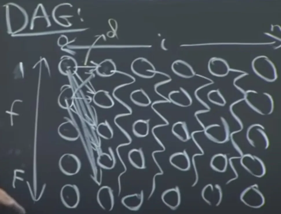
The columns represent the notes. The rows represent which finger to use. Each node in column i points to each node in column i+1.

Running time: O(n*F²), where F is the number of fingers. When small, this is basically linear time (e.g. 5 fingers leads to O(25n).

For guitar, there are multiple ways to play the same note depending on which string and fret. We could just generalize “finger” to “finger + string”.

Running time then becomes O(nF²S²) where S is the number of strings.

We can also generalize this to multiple notes. Before, the input was a sequence of notes. Now, notes[i] would represent a list of notes that you have to play all at once.

Running time becomes O(n * (F+1)^(2F))

Tetris

Artificial constraints:

We know the n pieces that are going to fall
Must move and rotate a piece while it’s “above” the board and then hard-drop the piece from the top, so there’s no moving or rotating them at the very end.
Full rows don’t clear, so you would lose eventually given enough pieces. The question is “will the N pieces fit in the board?”
Width of the board, w, is small
The board is initially empty

If we don’t know the n pieces that are going to fall, then this becomes NP-complete, meaning we can only verify the solution in polynomial time, but we can’t actually solve it in polynomial time unless we use a non-deterministic method.

Subproblems:
- Suffix of how to play pieces[i:]. However, we also need to know what the board looks like. We only need the “skyline” of the board since no rotations are allowed.
  - There are w columns and each can be up to h+1 choices, so it’s (h+1)^w.
  - We have n * (h+1)^w subproblems.
Guesses
- What should I do with piece i?
  - There are roughly 4 * w choices since there are 4 rotations and w coordinates where we could place the piece.

Total time complexity: O(n _ w _ (h+1)^w)

Our goal is to maximize whether we survived or not.

Super Mario Bros.

Given an entire level n
You have a small w * h screen
Configuration
- We care about everything on-screen: objects, enemies, etc. There’s c^(w*h) possibilities, where “c” is some constant.
- Mario’s velocity
- Score - S big
- Time - T big
- How far forward the screen has advanced in the level (“x”)

O(x * c^(w*h) _ S _ T)

The things we can do is push or release a button. Our subproblems are based on whether we’re trying to maximize score or minimize time.