Excel - Google Sheets

Created: 2015-08-06 21:28:32 -0700 Modified: 2022-01-30 10:18:14 -0800

Basics

Random tips in this giant reddit post here
For Google Sheets, you can use https://sheets.new/ to quickly make a new spreadsheet.

Misc

Here’s a very advanced FIRE spreadhseet with cool charts/tables (direct link)

8/6/2015

In Google Sheets, I had a column of numbers, and I wanted to take each element in the column, multiply by 2, and then put the result in the element just to the right.

E.g.

Before:

A	B
1
2
3

After:

A	B
1	2
2	4
3	6

To do this, I selected B2, typed “=A*2”, then a blue highlight box showed up with a little grabber at the bottom right. Just drag the grabber down for the whole column and it will copy the formula.

If you have part of the formula that should remain constant, e.g. referencing a lookup in another sheet, prefix it with a dollar sign (reference). So $A1 is a constant column, A$ 1 is a constant row, and $A$ 1 has both constant.

1/6/2016

In Google Sheets, if you click the “123” dropdown and choose a custom number format, you can make something like this:

+00”%“

This will format the number “50” as “+50%“. If you try doing this WITHOUT the number format, you’ll get weird results.

2/25/2016

To make a date range, just type out your first date in A1, e.g. 2/25/2016. Then, in the row below it (A2), type “=A1 + 7” to get the next Thursday. Then, select A2, copy it, then select A3 - A50 and paste. You’ll get every Thursday for as many weeks as you selected.

Referencing a cell in another sheet (<sheet name>!)

2/25/2016

To reference a cell in another sheet, you use “<sheet name>! $\<column\>$ <row>”, e.g. “=MyFirstSheet! $C$ 7” to pull from “MyFirstSheet” into the current cell.

If the sheet name has a space, surround it in single quotes: ‘Sheet with space’!B2

2/28/2016

Use colon for ranges. E.g. if you’re summing everything from B2 to B8, just do “=SUM(B2:B8 )“.

For “infinite” ranges, just use a letter with no number. E.g. C:C is all of column C. C2:C is all of column C after the first row.

5/27/2016

WeeDLY93 wanted to be able to get the name of a sheet so that he could access values in it to sum them up:

function AllValue(cell)

{

var ss = SpreadsheetApp.getActive();

var allSheets = ss.getSheets();

var sum = 0;

for(var s in allSheets)

{

var sheet = allSheets[s];

sum += sheet.getRange(cell).getValue();

}

return sum;

}

This would have worked if he didn’t mind specifying the sheet name though: =SUM(Sheet1! $A$ 1, Sheet2! $A$ 1)

Conditionally highlight dates based on elapsed number of days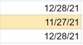

↑ Highlighted older dates yellow to indicate needing to update them

In this case, I clicked column C since that had my dates, then went to Format → Conditional formatting → Custom formula:

=AND(NOT(ISBLANK(C1)), DAYS(TODAY(), C1) > 14)

(C1 just refers to the given cell in the C column)

Finding which level you are based on current experience (reference)

(that’s easier to say than the generic case)

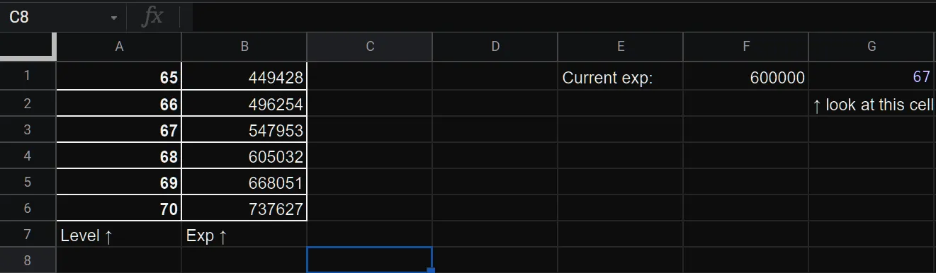
G1 is calculated by “=MINIFS(exp!A $1:A$ 6, exp!B $1:B$ 6, ”>=” & F1) - 1”

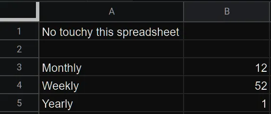
Lookups

I had a list of recurring transactions with a column for the frequency (weekly, monthly, or yearly). I wanted to figure out the yearly amount for all of them, so I made a “Lookups” sheet:

Then, to get the appropriate value, I wrote this:

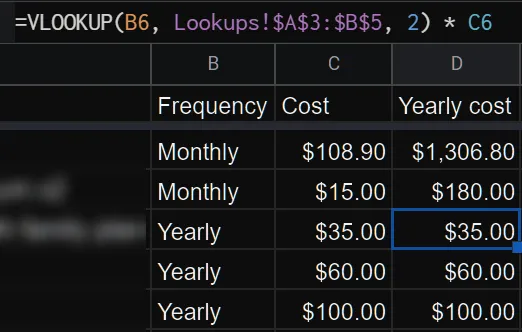
=VLOOKUP(B6, Lookups! $A$ 3: $B$ 5, 2) * C6